Parallel Predictive Bayes with CUDA

Those who have knowledge don’t predict. Those who predict don’t have knowledge. - Lao Tzu, badly translated

I’d like to share with you all a new perspective on Bayesian prediction that I learned from one of my professors recently. For the full description, check out the paper Martingale Posteriors (2021) by Edwin Fong, Chris Holmes, and Stephen G. Walker (the professor who taught me all this). For a brief introduction to the ideas in the paper, and also some code demonstrations using PyCuda, read along!

In my experience, Bayesian statistics lures people in with the simplicity of it’s paradigm. Every question you could possibly ask about a parameter is answered by its posterior distribution, which always going to pe proportion to the product of its likelihood and your prior expectations about it, elegantly summed up in the equation

This definition of the posterior underlies almost all Bayesian inference, perhaps to Bayesians’ own detriment (I even heard a joke last week from one of my colleagues that “Bayesians are all too preoccupied with their own posteriors”). One major benefit of posterior distributions on parameters is that instead of a simple point estimate and confidence interval, it can fully describe our uncertainty around a parameter. Uncertainty in an estimate of a parameter is property of the posterior distribution which basically tells us how wrong the estimate of the parameter could be and how likely it is to be that wrong.

Where does this uncertainty come from though? I had initially learned that uncertainty is essentially contained in the prior distribution imposed by the statistician. If I know nothing about the value of a parameter besides its range (for instance, $\theta \in [0,1]$), I may impose a $\text{Unif}(0,1)$ prior on it. But, as the Fong, Holmes, and Walker paper points out, this steps too far away from the true problem. Uncertainty about a parameter isn’t contained in a prior distribution designed to represent a statisticians expectations about it, it’s contained in the size of the sample! A parameter, after all, is a function of the population distribution $p(y_{1:\mathrm{\infty }})$. If we had an infinitely large sample we wouldn’t have any uncertainty about what the value of the parameter is, we could just calculate it with no need to predict or estimate!

This idea about the source of uncertainty is the core of this new paradigm I want to introduce y’all to. The big idea that comes from it is this: Why predict the parameter when instead we could predict the population and calculate the parameter?

Clearly, that won’t be as simple as I’m making it sound, but it could be simpler in practice than the Markov chain Monte Carlo (MCMC) methods out there. The basic procedure for sampling the population is this:

1. Sample a new observation from the predictive distribution $p_n(y)=p(y_{n+1}\mid y_{1:n})$.
2. Update the predictive distribution $p_{n+1}(y)=p(y_{n+2}\mid y_{1:n+1})$.
3. Repeat steps 1 and 2 some arbitrarily large number $N$ times.
4. Record $y_{1:n+N}$ as a new population sample and repeat steps 1-3 again some number $k$ times.

Now we have $k$ simulated populations on which we can compute $k$ possible values of the parameter $\theta$.

If the distribution of our $k$ sampled values of $\theta$ converges the correct posterior distribution, then this method could prove to be much faster to implement and to run than a conventional MCMC routine. First, because it’s easily parallelizable across the $k$ sampling chains and second, because there’s only one recursive update that needs to be programmed.

Now, using a trivial example, I want to show you that the distribution of $\theta$’s does in fact converge to the posterior distribution as well as demonstrate how this kind of sampling can be coded up and run. (If you want a proof, go check out the paper).

The example I’ll use is the same as that Example 1 in the paper. I wrote code to reproduce this example after talking to Stephen Walker about GPU programming and learning that he had recently been working on a sampling routine that lends itself very well to parallelization. This mini-project was actually my one of first exposures to CUDA!

The problem is structured like this:

Here, $y$ comes from a normal distribution with a known variance and unknown mean. We assign a standard normal prior on the mean which yields the posterior and posterior predictive distributions:

where

Now, lets write some code to implement predictive resampling in parallel on a GPU and compare the resulting distribution of $\theta$ to its posterior. In CUDA, the global kernel function will look as follows:

#include <curand_kernel.h>

extern "C"
{
    __global__ void resampler(float *dest, int *iparams, float *fparams, curandState *global_state)
    {
        /* Set chain parameters */
        const int idx = blockDim.x * blockIdx.x + threadIdx.x;
        const int m = threadIdx.x;
        const int n_iter = iparams[0];

        /* Set sampling parameters */
        float theta = fparams[0];
        float n = fparams[1];

        /* Initialize local_state */
        curandState local_state = global_state[m];
        curand_init(idx, idx, idx, &local_state);

        /* Open sampling loop */
        for (int iter = 0; iter < n_iter; iter++)
        {
            /* Draw y */
            float y = theta + curand_normal(&local_state) / sqrt(1 + 1 / (n + 1));

            /* Update params */
            theta = (theta * (n + 1) + y) / (n + 2);
            n = n + 1;

            /* Record estimate of theta */
            dest[(idx) * n_iter + iter] = theta;

            /* Update local state */
            global_state[m] = local_state;
        }
        
    }
}

Here, we have a function which takes as arguments a destination array (for copying results), an array of integer parameters (for $N$), an array of floating point parameters (for and initial estimate of $\theta$ and sample size $n$ (which is type-cast as a floating point to preempt division issues)), and a global random state for random variate generation. In the sampling loop, it draws a new observation $y$ given the estimate of the mean $\theta$ conditioned on all the previously sampled values of $y$, then updates $\theta$ with this new value of $y$ and records it in the destination. This updating process is repeated $N$ times for each thread opened by the GPU.

To run this code, I decided to compile it with PyCUDA since I wasn’t yet ready to work with the explicit memory allocation required in CUDA. In PyCUDA, I could simply save the above code as a string in Python and pass it to PyCUDA’s SourceModule function. I’ll include all the Python code at the end of this post.

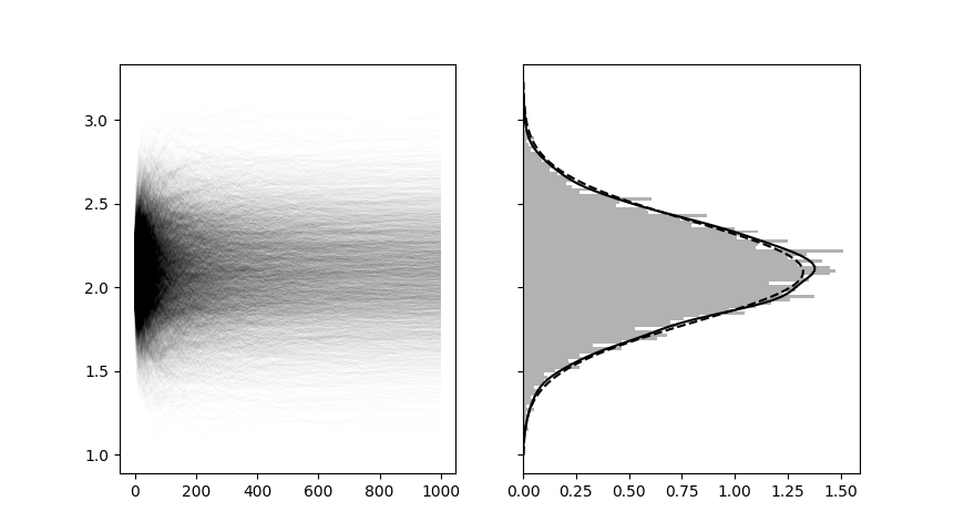
Using a true value of $\theta =2$ I ran the above kernel $k=4096$ times with each thread simulating $N=1000$ unobserved values of $y$ into the future. Thanks to GPU parallelization, several hundred and possibly thousands of these threads were able to run concurrently (I’m still learning about CUDA’s scheduling protocol to learn exactly how many threads are running at once). The compilation of the CUDA kernel took 1.8 seconds, but the actual simulation of 4,096,000 possible unobserved $y$ values took 0.025 seconds. The plot below shows the sampling trajectories of each of the 4096 $\theta$’s and the distribution of $\theta$ values at the 1000th predictive resample. The true posterior is included in dashed black.

Here, y-axis represents the estimated values of $\theta$ and the x-axis for the left hand side shows the number of unobserved values simulated. The x-axis for the right hand side is simple a density measure.

Now, clearly this is a very simple example and you may not believe me that, in general, this practice will always give you samples from the posterior at a large enough $N$. As I said before, check the paper for a formal proof (and find out why they call them “Martingale posteriors”!).

All I wanted to show here was how efficiently – and honestly how simply – these recursive predictive updates can be implemented. In this example, there was still a heavy focus on the prior and posterior distributions of $\theta$, but in my next post I plan to show you how we can generalize this approach into a nonparametric predictive resampling regime by using a special family of distributions called “copulas”, and of course there will be another code demo. I know today’s demo was a much less descriptive than it should have been, but I’ve been super slow getting this post out and I figured I’d just rip off the bandaid and post it the way it is before it ends up in the backlog for a year. Leave a comment for me below if you want me to make the code more clear for you, or if you think I should focus more on the code than the math next time around!

Anyway, I’ll see you next time for more predictive Bayes.

Thank you,
Blake

• Previous
  A Return to Blogging